Calculus III:

Line integrals with respect to arc length ds

1. Definition and method

Integrating a function of a single variable f(x) over an interval [a,b], x takes all the values in this interval starting at a and ending at b.

Double-integrating a function of a two variable f(x,y) over a domain [a,b] D, x and y take all the values in this domain starting at a and ending at b for x; and starting atc and ending at d for y.

With line integrals we integrate the function f(x,y), a function of two variables, and the values of x and y will be the points, (x,y), that lie on a curve C.

Notice that this is different from the double integrals where the integration is made over a region R or D. In line integrals, we integrate over a curve made from the points of the the function itself.

Let’s consider the curve C that the points come from, and assume assume that the curve is smooth. The curve is given by the parametric equations:

x = g(t), y = h(t)       a ≤ t ≤ b

With the parameterization of the curve as a vector function, the curve is given by:

(t) = g(t) + h(t)       a ≤ t ≤ b

Let's recall that the curve is called smooth if(t) is continuous and(t) ≠ for all t.

The line integral of f(x,y) along C is denoted by:



The differential element is ds. This is the fact that we are moving along the curve, C, instead dx for the x-axis, or dy for the y-axis.

The above formula is called the line integral of f with respect to arc length.

Let's recall that the arc length of a curve is given by the parametric equations:

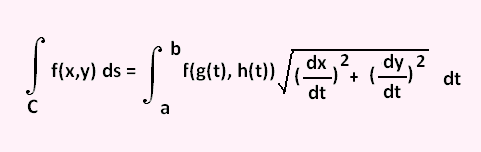
L = ∫_a^b ds   width   ds = √[(dx/dt)² + (dy/dt)²] dt

Therefore, to compute a line integral we convert everything over to the parametric equations. The line integral is then:

Example 1

Evaluate ∫_C 3x² ds where C is the line segment from (-1, 1) to (1,2).

We have already seen, in the equation of a line in 3D space section, that the parameterization formula of the line segment starting at the point(xo, yo) and ending at the point (x1,y1) is :

(t) = (1 - t) 〈xo, yo〉 + t 〈x1,x2〉

That is:

x = xo (1 - t) + x1 t
y = yo (1 - t) + y1 t



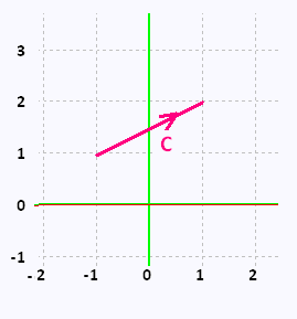
So, the parameterization formula of the line segment starting at (-1, -1) and ending at (1,2) is :

(t) = (1 - t) 〈-1, 1〉 + t 〈1,2〉.

That is:

x = (1 - t) (- 1) + t(1) = 2t - 1
y = (1 - t) (1) + t(2) = t + 1

At (-1, 1): x = - 1, y = 1 → t = 0 , and
at (1,2): x = 1 , y = 2 → t = 1

so 0 ≤ t ≤ 1

We have: dx/dt = 2 , and dy/dt = 1. Hence:
ds = √[2² + 1²] dt = √5 dt.

ds = √5 dt

Therefore

∫_C 3x² ds = ∫₀¹ 3(2t - 1)² √5 dt = 3 √5 ∫₀¹ (4t² - 4t + 1) dt =
3√5 [(4/3)t³ - 2t² + t] ₀¹ = 3√5 [(4/3) - 2 + 1] =
3√5 [1/3] = √5

∫_C 3x² = √5

Example 2

Evaluate ∫_Cxy² ds where C is the right half of the circle x²+ y² = 16, rotated in the counter clockwise direction.



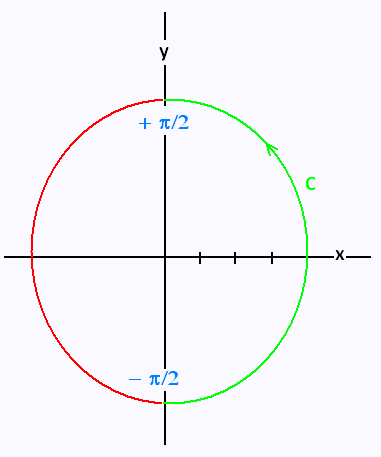
We parameterize the curve which is the circle, then the integrand, and then the differial element:

x = 4 cos t, y = 4 sin t     - π/2 ≤ t ≤ + π/2.

f(x,y) = xy² = 4 cos t (4 sint)² = 64 cos t sin²t

dx/dt = - 4 sin t , dy/dt = 4 cos t

ds = 4 dt

Therefore

∫_C xy² ds = ∫_{- Ï€/2} ^{+ Ï€/2} 64 cos t sin²t (4 dt) =
256 ∫_{- Ï€/2} ^{+ Ï€/2} cos t sin²t dt = 256 [(1/3) sin³ t]_{- Ï€/2} ^{+ Ï€/2} =
(256/3)[sin³ (Ï€/2) - sin³ (-Ï€/2)] = 2 (256/3) sin³ (+ Ï€/2) = 2 (256/3) = 512/3.

∫_C xy² ds = 512/3

2. Integrals over piecewise smooth curves

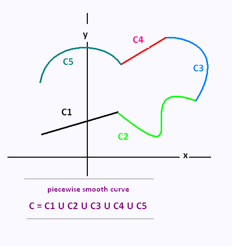
Now, we are going to integrate line integrals over piecewise smooth curves.

A piecewise smooth curve C is any curve that can be written as the union of a finite number of smooth curves, C1, C2, C3, , ... Cn, where the end point of Ci is the starting point of Ci+1.

To evaluate the line integrals over piecewise smooth curves , we evaluate the line integral over each of the pieces and then add them up:

∫_C f(x,y) ds = ∫_C1 f(x,y) ds ∫_C2 f(x,y) ds ∫_C3 f(x,y) ds ∫_C4 f(x,y) ds ∫_C5 f(x,y) ds + ...

Example 3

Evaluate ∫_C 2x ds
where C is the curve shown below.


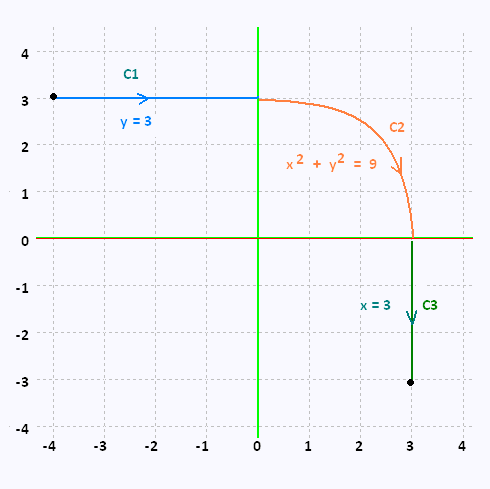
C1: x = t , y = 3     - 4 ≤ t ≤ 0

C2: x = 3 cos t , y = 3 sin t     π/2 ≤ t ≤ 0

C3: x = 3 , y = t     - 3 ≤ t ≤ 0

C1:

dx/dt = 1    dy/dt = 0
ds = dt

∫_C1 2x ds = ∫_{- 4}⁰ 2t dt = (t²)|_{- 4}⁰ = 16

∫_C1 2x ds = 16

C2:

dx/dt = - 3 sint    dy/dt = 3 coos t
ds = 3 dt

∫_C2 2x ds = ∫_Ï€/2⁰ 2 cos t (3 dt) = 6 (sin t)|_Ï€/2⁰ = 6 (sin t)|_Ï€/2⁰ = - 6

∫_C2 2x ds = - 6

C3:

dx/dt = 0    dy/dt = 1
ds = dt

∫_C3 2x ds = ∫₀^-3 2 (3) dt = 6 (t)|₀^-3 = 6(- 3) = - 18

∫_C3 2x ds = - 18

Therefore:

∫_C 2x ds = ∫_C1 2x ds + ∫_C2 2x ds + ∫_C3 2x ds .

= 16 - 6 - 18 = - 8

∫_C 2x ds = - 8

Example 4

In the example 1, we have have found:

∫_C 3x² ds where C is the line segment from (-1, 1) to (1,2).

Here we switch the direction of the curve to see whether le liine integral change:

We evaluate Then ∫_-C 3x² ds where -C is the line segment from (1,2) (- 1, 1).

The parameterization formula of the line segment starting at (1, 2) and ending at (- 1, 1) is :

(t) = (1 - t) 〈1, 2〉 + t 〈- 1,1〉.

That is:

x = (1 - t) (1) + t(- 1) = 1 - 2t
y = (1 - t) (2) + t(1) = 2 - t

At (1,2): x = 1 , y = 2 → t = 0 , and
At (-1, 1): x = - 1, y = 1 → t = 1

so 0 ≤ t ≤ 1

We have: dx/dt = - 2 , and dy/dt = - 1. Hence:
ds = √[2² + 1²] dt = √5 dt.

ds = √5 dt

Therefore

∫_-C 3x² ds = ∫₀¹ 3(1 - 2t)² √5 dt = √5

∫_-C 3x² = √5 , as in the example 1.

So, for this kind of line integrals, that is for the integrals with respect to the arc length ds , when we switch the direction of the curve, the line integral (with respect to arc length) will not change. But it does not hold for all the line integrals. For a line integrals with respect to arc length, we have:

∫_C f(x,y) ds = ∫_-C f(x,y) ds

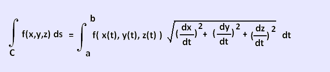
3. Line integrals over a three-dimensional curve

The line integrals over a three-dimensional curve can be extended from the line integrals over atwo-dimensional curve.

Let’s suppose that the three-dimensional curve C is given by the parameterization:

x = x(t), y = y(t), z = z(t)     a ≤ t ≤ b.

The line integral is then given by: