Calculus III
Contents
3 Dimensional space
Partial derivatives
Multiple integrals
Vector Functions
Line integrals
Surface integrals
Vector operators
Applications
© The scientific sentence. 2010
|
|
Calculus III:
Green�s Theorem
Green�s Theorem involves:
• two-dimension space,
• line integrals on simple closed paths,
• region enclosed by the curve,
• double integrals,
• no vectors,
• ∮ or positively oriented ∳
1. Green�s Theorem
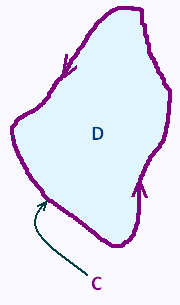
Let�s consider a simple closed curve C and let D be the region enclosed by this curve.
The curve C is simple, that is, it does not cross itself. Also, the
curve has a positive orientation, that is a counter-clockwise direction
(region D must be on the left) has been put on the curve.
The region D does not contain holes because the curve is simple and closed.
In these conditions, we have the following theorem:
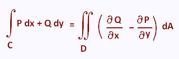
Let C be a positively oriented, piecewise smooth, simple, closed curve and let D be the region enclosed by the curve. If P and Q have continuous first order partial derivatives on D then:
When the path satisfies the conditions of Green�s Theorem we denote
often the integral symbol with ∮ or ∳.
Example 1
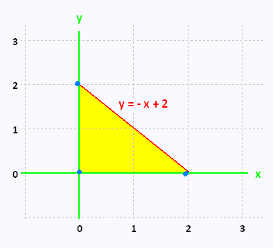
Evaluate ∳C (1/2)y2x dx + x2y dy,
by using Green�s Theorem. C is the triangle with vertices (0,0), (2,0) (0,2) with positive orientation.
Let�s sketch the curve C and the region D to make sure that the conditions of Green�s Theorem are met. C is the contour formed by the three sides of the
triangle, and D is the surface of the triangle where to evaluate the double integral.
We have:
P(x,y) = (1/2)y2x
Q(x,y) = x2y
The partial derivative are:
∂P/∂y = xy
∂Q/∂x = 2xy
∂Q/∂x - ∂P/∂y = 2xy - xy = xy
The region enclosed is then defined by the following inequalities:
0 ≤ x ≤ 2
0 ≤ y ≤ 2-x
Therefore
∫∫D(∂Q/∂x - ∂P/∂y) dA =
∫02
∫02-x
(xy) dy dx =
∫02
(1/2)x(2 - x)2
dx =
(1/2)∫02
(x3 - 4x2 + 4x)
dx =
(1/2)∫02
((1/4)x4 - (4/3)x3 + 2x2)
dx =
(1/2)(4 - 32/3 + 8) =
2/3.
∳C (1/2)y2x dx + x2y dy = 2/3
Example 2
Evaluate ∳C yx2 dx - xy2 dy,
where C is the positively oriented circle of radius 2 centered at the origin.
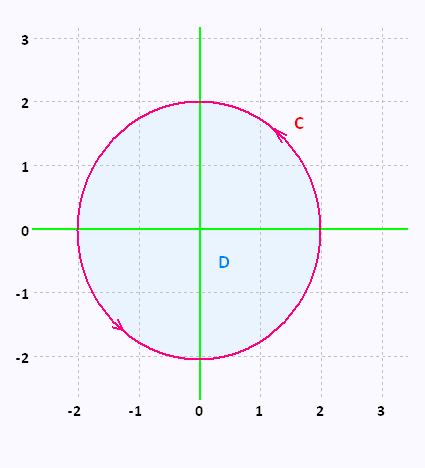
The circle C satisfies the conditions of Green�s Theorem since it is closed and simple and so define a region D which is the disc of radius 2.
We have:
P(x,y) = yx2 and
Q(x,y) = - xy2
The partial derivative are:
∂P/∂y = x2 and
∂Q/∂x = - y2
∂Q/∂x - ∂P/∂y = - y2 - x2 =
- (x2 + y2)
So, using Green�s Theorem, with the parameterization x = r cosθ and
y = r sinθ, the line integral becomes:
∳C yx2 dx - xy2 dy =
∫∫D - (x2 + y2) dA =
∫02
∫02π dθ (- r3) dr =
2π
(- (1/4) r4)|02 = - 8 π
∳C yx2 dx - xy2 dy =
- 8 π
2. Splitting enclosed regions
Green�s theorem is stated on regions that don't have holes in them. However, many regions used do have holes in them. So, we will workaround
by splitting the given region with holes into two or more other other
enclosed regions.
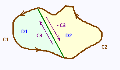
Let�s consider the following region that doesn�t have any holes in it. We
split it into two regions D1 and D2 by adding two boundaries C3 and - C3
that cancel each other out.
D = D1 ∪ D2
The contour of D1 is C1 ∪ C3. The contour of D2 is C2 ∪ - C3.
All the countours C1, C3, C2, and - C3 are positively
oriented.
The whole contour C is :
C = C1 ∪ C2 = C1 ∪ C3 ∪ - C3 ∪ C2
The double integral over D is the broken up in D1 and D2:
∫∫D (Qx - Py) dA
= ∫∫D1∪D2 (Qx - Py) dA
= ∫D1 (Qx - Py) dA
+
∫D2 (Qx - Py) dA =
Using Green�s theorem on each of these , we obtain:
= ∳C1∪C3 P dx + Q dy
+
∳C2∪-C3 P dx + Q dy
Again breaking these line integrals up into separate line integrals for each portion of the contour, we obtain:
= ∳C1 P dx + Q dy +
∳C3 P dx + Q dy
+
∳C2 P dx + Q dy +
∳-C3 P dx + Q dy
Using the formula:
∳-C3 P dx + Q dy = - ∳C3 P dx + Q dy,
We get:
∳C1 P dx + Q dy
+
∳C2 P dx + Q dy
=
∳C1∪C2 P dx + Q dy
=
∳C P dx + Q dy
Therefore
∫∫D (Qx - Py) dA =
∳C P dx + Q dy
Conclusion
If we break a region up, then the duilt portions of the line integral cancel out.
This is an important property to determine line integrals over
a region that have holes de in them.
3 . Green's theorem on regions with holes
Let's consider a ring between two circualr contours.
Both of the curves C1 and C2 are oriented positively. To check this,
for C1, the region D is on the left side as we traverse the curve in the indicated counter-clockwise direction.
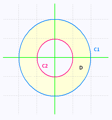
The curve C2 is the contour of the hole . Its positive orientation
is in a clockwise direction; in order to have the region at left.
Now, the given region has a hole in it. So, we cannot use Green�s Theorem on
it. To use then Green's theorem, we have to modify it this way:
we cut the disk in half. With the four built new portions C3, -C3, C4, and - C4, we get the following contour:
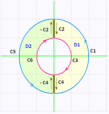
The contour of the right portion (D1) of the disk is
C1∪C2∪C3∪C4; and the contour on the left
portion (D2) of the disk is C5∪-C4∪C6∪-C2 .
We can use Green�s Theorem on each of these
new regions D1 and D2 since they don�t have any holes in them.
Therefore
∫∫D (Qx - Py) dA =
∫∫D1 (Qx - Py) dA +
∫∫D2 (Qx - Py) dA
=
∳C1∪C2∪C3∪C4 P dx + Q dy +
∳C5∪-C4∪C6∪-C2 P dx + Q dy
=
∳C1 P dx + Q dy +
∳C2 P dx + Q dy +
∳C3 P dx + Q dy +
∳C4 P dx + Q dy +
∳C5 P dx + Q dy +
∳-C4 P dx + Q dy +
∳C6 P dx + Q dy +
∳-C2 P dx + Q dy
=
∳C1 P dx + Q dy +
∳C3 P dx + Q dy +
∳C5 P dx + Q dy +
∳C6 P dx + Q dy
=
∳C1 P dx + Q dy +
∳C5 P dx + Q dy +
∳C3 P dx + Q dy +
∳C6 P dx + Q dy
= ∳outer contour counter-clockwise P dx + Q dy +
∳inner contour clockwise P dx + Q dy
=
= ∳outer contour counter-clockwise P dx + Q dy +
- ∳inner contour counter-clockwise P dx + Q dy
Therefore
∫∫D (Qx - Py) dA =
∳outer contour counter-clockwise P dx + Q dy
- ∳inner contour counter-clockwise P dx + Q dy
Example 3
Evaluate ∳C yx2 dx - xy2 dy,
where C are the two circles C1 and C2 of radius 2 and 1
respectively, centered at the origin with positive orientation.
We have:
P(x,y) = yx2 and
Q(x,y) = - xy2
The partial derivative are:
∂P/∂y = x2 and
∂Q/∂x = - y2
∂Q/∂x - ∂P/∂y = - y2 - x2 =
- (x2 + y2)
So, using Green�s Theorem, with the parameterization x = r cosθ and
y = r sinθ, the line integral becomes:
∳C1-C2 yx2 dx - xy2 dy =
∫∫D - (x2 + y2) dA =
∳C1 yx2 dx - xy2 dy -
∳C2 yx2 dx - xy2 dy
∳C1 yx2 dx - xy2 dy = - 8 π
∳C2 yx2 dx - xy2 dy = - π/2
Therefore
∳C1 yx2 dx - xy2 dy -
∳C2 yx2 dx - xy2 dy =
- 8 π - (- π/2) = - 15π/2
∳C yx2 dx - xy2 dy = - 15π/2
4. Green's theorem : application
the area of a region D
The area of a region D is determined with the following double integral:
A = ∫∫D dA
In order to use Green�s Theorem , we will have:
Qx- Py = 1
There are many functions that will satisfy this.
Here are some of them:
Qx = 1 and Py = 0, or
Qx = 0 and Py = - 1, or
Qx = 1/2 and Py = - 1/2
That is
Q = x and P = 0, or
Q = 0 and P = - y, or
Q = x/2 and P = - y/2
Therefore
A = ∳C x dy = - ∳C y dx =
(1/2)∳C x dy - y dx
Where C is the boundary of the region D.
Example 4
We want to use Green�s Theorem to find the area of a disk of radius a.
We can use either of the integrals above.
A = (1/2)∳C x dy - y dx
where C is the circle of radius a.
A parameterization of C gives:
x = a cos t , y = a sin t 0 ≤ t ≤ 2π
Then
dx = - a sin t dt , and dy = a cos t dt
Therefore
A = (1/2)∳C x dy - y dx =
(1/2)∫0 2π a2 cos2 t + a2 sin2 t dt =
(1/2) 2 π a2 = π a2 .
The area is then
A = π a2
5. Three-dimentional form of Green's theorem
• Using the curl of the vector field  : :
∳C .  =
∫∫D (curl ) . =
∫∫D (curl ) .  dA dA
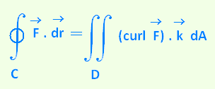
is the standard unit vector in the positive z direction.
• Using the divergence of the vector field :
∳C.  ds =
∫∫D (div ) dA ds =
∫∫D (div ) dA
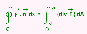
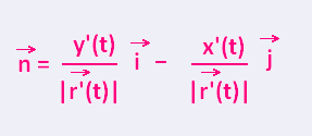
is the outward unit normal vector to the curve C.
If the curve is parameterized by
 (t) =
x(t) (t) =
x(t)  + y(t) + y(t)  ,
we will have: ,
we will have:
 = x'(t) + y'(t) , and = x'(t) + y'(t) , and
= (y'(t)/|(t)|) -
(x'(t)/|(t)|)
|
|